Shipgrav
Introduction
shipgrav is a Python package with utilities for reading and processing marine gravity data from UNOLS ships. At time of writing, the UNOLS fleet is transitioning away from BGM3 gravimeters to DGS AT1M meters managed by the Potential Field Pool Equipment (PFPE) facility. shipgrav is able to read files from both types of meters, as well as navigation data and other vessel feeds. shipgrav functions can then be used to process gravity data to FAA, MBA, RMBA, and crustal thickness estimates.
DGS gravimeters output two types of files: serial, or ‘raw’ files; and ‘laptop’ files. Raw files are written from the serial port, and contain counts values that can be calibrated to retrieve the gravity signal. In this documentation we use the terms ‘serial’ and ‘raw’ interchangeably. What we refer to as laptop files are lightly processed onboard the meter and output with (biased) gravity values alongside other information.
Installation
shipgrav can be installed from PyPI using pip. We recommend using an environment management tool like conda. An exemplary set of commands to make a conda enviroment with shipgrav would be:
conda create --name shipgrav numpy scipy pandas statsmodels tomli pyyaml tqdm pooch matplotlib geographiclib
conda activate shipgrav
pip install shipgrav
shipgrav’s dependencies are
Python 3.9+
numpy
scipy
pandas 2.0+
statsmodels
tomli
pyyaml
tqdm
pooch (optional, needed to run the example scripts)
matplotlib (optional, needed to run some of the example scripts)
geographiclib (optional, needed to run one of the example scripts)
jupyterlab (optional, if you want to run example scripts in jupyter)
jupytext (optional, if you want to run example scripts in jupyter)
If you install shipgrav with pip, it will also install any of the required dependencies that are missing. To make pip include the optional dependencies, run pip install shipgrav[examples]. Depending on your operating system and shell, you may need to escape the brackets (i.e. pip install shipgrav\[examples\]).
The example scripts are available on github. They are not packaged with the PyPI package and must be downloaded separately.
Modules and files
shipgrav consists of the modules io, nav, grav, and utils, along with the file database.toml and a set of example scripts.
iocontains functions for reading different kinds of gravimeter files and associated navigation files.navcontains functions for handling coordinate systems.gravcontains functions for processing gravity data and calculating various anomalies.utilsis a catch-all of other things we need.database.tomlholds some ship-specific constants and other information for UNOLS vessels.the scripts in
example-scripts/walk through the steps of reading and processing UNOLS gravimeter data for a set of data files that are publicly available via R2R (Rolling Deck to Repository).
Data directories
You can organize your data however you like; shipgrav does not care as long as you tell it where to look. The example scripts are set up to download data files from public repositories using pooch. The pooch.retrieve() function returns lists of file paths for files that have been downloaded and unpacked, so to adapt the example workflows for other data files, you will need to replace those lists of paths with the paths to your data.
Ties and bias
The database.toml file contains some bias values for UNOLS vessels. These are provided for your convenience, but are not necessarily up-to-date with recent gravity ties.
Example scripts
The scripts in the example-scripts/ directory use publicly available data files to run through some common workflows for marine gravity processing. All of the examples can be run as scripts (ie, with python -m <script-name>.py). All except interactive_line_pick.py can also be opened in jupyter as notebooks thanks to jupytext. To run the examples in jupyter, start jupyter lab, right-click on the script file name, and select open with -> notebook.
The data files can be downloaded from R2R and Zenodo, and the scripts will do this automatically using pooch. The sources are:
https://doi.org/10.7284/151470 - TN400 BGM3 data
https://doi.org/10.7284/151457 - TN400 nav data
https://doi.org/10.7284/157179 - SR2312 DGS laptop data
https://doi.org/10.7284/157188 - SR2312 nav data
https://doi.org/10.7284/157177 - SR2312 mru data
https://doi.org/10.5281/zenodo.12733929 - TN400 DGS raw and laptop data, SR2312 DGS raw data, R/V Ride DGS meter and Hydrins metadata, satellite FAA tracks for comparison, example file for RMBA calculation
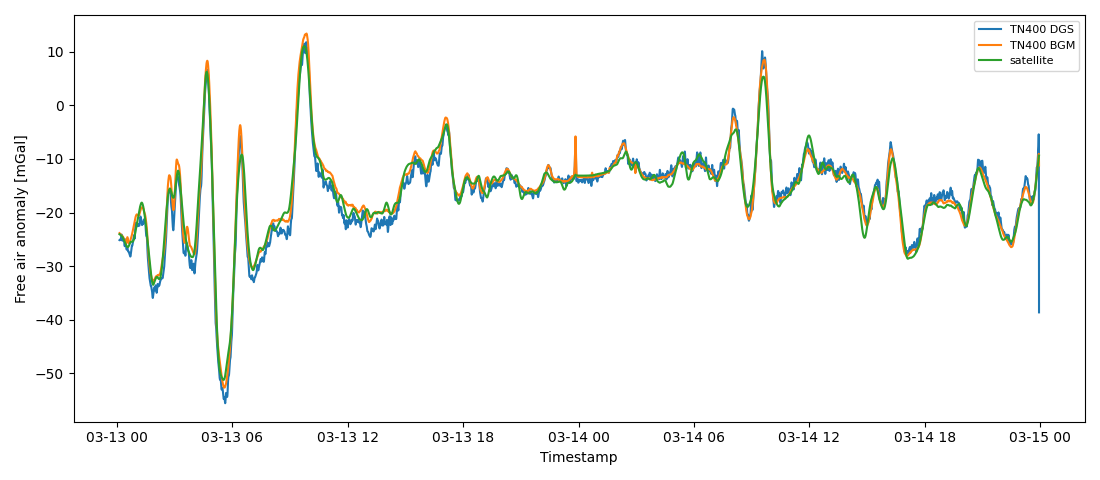
dgs_bgm_comp.py reads data from DGS and BGM gravimeter files from R/V Thompson cruise TN400. The files are lightly processed to obtain the FAA (including syncing with navigation data for more accurate locations), and the FAA is plotted alongside corresponding satellite-derived FAA.
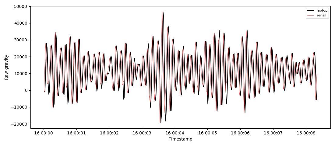
dgs_raw_comp.py reads laptop and serial data from R/V Sally Ride cruise SR2312. The serial data are calibrated and compared to the laptop data. The laptop data are processed to FAA and plotted alongside satellite-derived FAA.
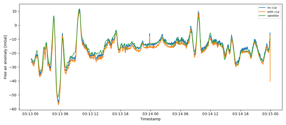
dgs_ccp_calc.py reads DGS files from R/V Thompson cruise TN400, calculates the FAA and various kinematic variables, and fits for cross-coupling coefficients. The cross-coupling correction is applied and the data are plotted with and without correction. Satellite-derived FAA is also plotted
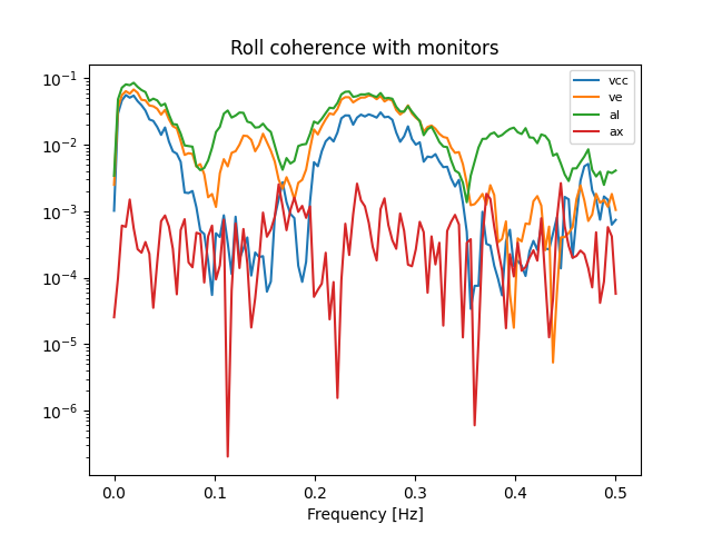
mru_coherence.py reads laptop data and other feeds from R/V Sally Ride cruise SR2312. The FAA is calculated, and MRU info is read to obtain time series of pitch, roll, and heave. Coherence is caluclated between those and each of the four monitors output by the gravimeter for the cross-coupling correction.
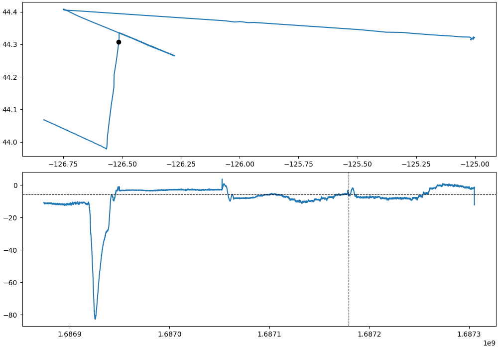
interactive_line_pick.py reads laptop data and navigation data from R/V Sally Ride cruise SR2312. The script generates an interactive plot with a cursor for users to select segments of the time series data based on mapped locations, in order to extract straight line segments from a cruise track. This script cannot be run in jupyter. The selected segments are written to files that can be re-read by the next script…
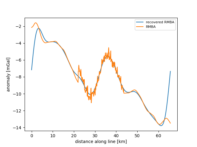
RMBA_calc.py reads an example of data from a line segment (from the interactive line picker) and calculates the residual mantle bouger anomaly (RMBA) as well as estimated crustal thickness variations.
Help!
FileNotFound errors: check the filepaths in your scripts and make sure that (a) there are no typos, and (b) you are pointing toward the actual locations of your data files.
Other file reading errors: shipgrav does its best to read a variety of file formats from UNOLS gravimeters, but we can’t read files that we don’t know enough about ahead of time. In some cases, a file cannot be read because we don’t yet know how to pass the file to the correct parsing function. Most primary i/o functions in shipgrav have an option where users can supply their own file-parsing function, so one option is to write such a function (following the examples in shipgrav for known vessel file formats) and plug that in via the appropriate kwarg (usually named ship_function). You can also send an example file and information to PFPE so that we can update shipgrav.
The anomaly I’ve calculated looks really weird: a good first step is to compare your (lowpass filtered) FAA to satellite data (e.g., Sandwell et al. 2014). If that looks very different, you can start checking whether the data is being read properly; whether the sample rate of the data is consistent with your expectations; whether there are anomalous spikes or dropouts in the data that need to be cleaned out; and whether the corrections used to calculate the FAA seem to have reasonable magnitudes.
I want to use shipgrav, but my data is not from a UNOLS vessel: the functions and workflows in shipgrav are entirely adaptable to use with data from other sources. You will need to determine the data format for your gravimeter files, and write or adapt a function to read that data. There are examples in the io module. If you have raw data files, you will also need to know the calibration constants and apply those. Once the data have been read (and calibrated), you should be able to apply all of the other shipgrav functions for processing.
I’m going to sea and want to be able to access this documentation offline: this is all auto-generated from text included in the shipgrav source files! So one option is just to go read those (the main part of the documentation is in shipgrav/__init__.py). To view it as a nice webpage, you can build the documentation locally using sphinx. Install sphinx in your conda environment, run the command make html in the docs/ directory, and then open docs/_build/html/index.html in your browser to view the documentation.
If you have some other question that’s not answered here: you can try contacting PFPE at pfpe-internal(at)whoi.edu for specific assistance with processing UNOLS gravimeter data.
Testing
shipgrav comes with a set of unit tests. To run them for yourself, navigate to the tests/ directory and run __main__.py (in an environment with dependencies installed, naturally).
Contributing
Do you have ideas for making this software better? Go ahead and raise an issue on the github page or, if you’re a savvy Python programmer, submit a pull request. You can also email PFPE at pfpe-interal(at)whoi.edu.
If you raise an issue on github, please include as much detail as possible, such as the text of error messages. If there are no visible errors but you think the code is behaving oddly, provide a description of what the code is doing and what you think it should be doing instead. PFPE may ask for additional details or copies of data files in order to reproduce and diagnose an issue.
API Reference
io Module
- shipgrav.io.read_bgm_raw(fp, ship, scale=None, ship_function=None, progressbar=True)
Read BGM gravity from raw (serial) files (not RGS).
This function uses scale factors determined for specific BGM meters to convert counts from the raw files to raw gravity. Known scale factors are listed in database.toml.
- Parameters:
fp (string or list of strings) – BGM raw filepath(s)
ship (string) – ship name
scale (float, optional) – BGM counts scaling factor to override database.toml
ship_function (function, optional) – user-supplied function for reading/parsing BGM raw files. The function should return a pandas.DataFrame with timestamps and counts. Look at _bgmserial_Atlantis() and similar functions for examples.
progressbar (bool) – display progress bar while list of files is read
- Returns:
(pd.DataFrame) timestamps and calibrated raw gravity values
- shipgrav.io.read_bgm_rgs(fp, ship, progressbar=True)
Read BGM gravity from RGS files.
RGS is supposedly a standard format; is consistent between Atlantis and NBP at least.
- Parameters:
fp (string, or list of strings) – RGS filepath(s)
ship (string) – ship name
progressbar (bool) – display progress bar while list of files is read
- Returns:
(pd.DataFrame) timestamps, raw gravity, and geographic coordinates
- shipgrav.io.read_dgs_laptop(fp, ship, ship_function=None, progressbar=True)
Read DGS ‘laptop’ file(s), usually written as .dat files.
- Parameters:
fp (string or list of strings) – filepath(s)
ship (string) – ship name
ship_function (function, optional) – user-defined function for reading a file. The function should return a pandas.DataFrame. See _dgs_laptop_general() for an example.
progressbar (bool) – display progress bar while list of files is read
- Returns:
(pd.DataFrame) DGS output time series
- shipgrav.io.read_dgs_raw(fp, ship, scale_ccp=True, progressbar=True)
Read raw (serial) output files from DGS AT1M.
These will be in AD units mostly. File formatting is assumed to follow what the DGS documentation says, though some things may vary by vessel so if this doesn’t work that’s probably why.
- Parameters:
fp (string or list of strings) – filepath(s)
ship (string) – ship name
progressbar (bool) – display progress bar while list of files is read
- Returns:
(pd.DataFrame) DGS output time series
Read navigation strings from .GPS (or similar) files.
Ships have different formats and use different talkers for preferred navigation; the ones we know are listed in database.toml, and there is also an option to override that by setting the talker kwarg. Navigation data is re-interpolated to the given sampling rate.
- Parameters:
ship (string) – name of the ship
pathlist (list, strings) – paths to navigation files (.GPS)
sampling (float) – sampling rate to interpolate to, default 1 Hz
talker (string, optional) – nav talker. Default behavior is to use talker from database.toml if ship is listed there.
ship_function (function, optional) – user-supplied function for reading from nav files. This function should return arrays of lon, lat, and timestamps. Look at _navcoords() and navdate_Atlantis() (and similar functions) for examples.
decimate (int, optional) – integer skip for decimating data, default 0 returns all points
progressbar (bool) – display progress bar while list of files is read
- Returns:
(pd.DataFrame) time series of geographic coordinates and timestamps
- shipgrav.io.read_other_stuff(yaml_file, data_file, tag)
Read a particular feed (eg, $PASHR) from a data file + yaml file.
This function parses strings for the desired feed and returns info as a pandas.DataFrame with columns named from the corresponding yaml file. If there is a column in the feed strings prior to the tag itself, that will be included as a ‘mystery’ dataframe column.
A use case is if you want to check coherence between gravity data and one or more MRUs
- Parameters:
yaml_file (string) – path to YAML file with info for this feed
data_file (string) – path to data file to be read
tag (string) – the name of the feed, with or without the $ prepended
- Returns:
(pd.DataFrame) time series from specified feed
grav Module
- shipgrav.grav.calc_cross_coupling_coefficients(faa_in, vcc_in, ve_in, al_in, ax_in, level_in, times=None, samplerate=1)
Calculate cross-coupling coefficients from FAA via ordinary linear regression
The cross-coupling coefficients are returned in model, in the params attribute
- Parameters:
faa_in (array_like) – free air anomaly, filtered
vcc_in (array_like) – vcc monitor
ve_in (array_like) – ve monitor
al_in (array_like) – al monitor
ax_in (array_like) – ax monitor
level_in (array_like) – tilt/leveling correction, often negligible. Use a vector of zeros to ignore this component.
times (array_like, floats, optional) – timestamps to use for dividing the data into continuous sections
samplerate (float, optional) – used with times to detect large sampling gaps in the data
- Returns:
df (pd.DataFrame)- double-differenced and filtered monitors and gravity
model (statsmodels.OLS)- linear regression model
- shipgrav.grav.center_diff(y, n, samp)
Numerical derivatives, central difference of nth order
- Parameters:
y (array_like) – data to differentiate
n (int) – order, either 1 or 2
samp (float) – sampling rate
- Returns:
1st or 2nd order derivative of y
- shipgrav.grav.crustal_thickness_2D(ur, nx=1000, ny=1, dx=1.3, dy=0, zdown=10, rho=0.4, wlarge=45, wsmall=25, back=False)
Downward continuation of gravity to “topographic relief” ie crustal thickness
This can be used in 2D, but also works for a single line given ny=1 (which is the default)
- Parameters:
ur (array_like) – residual gravity anomaly, mgal
nx (int) – number of points in x direction, default 1000
ny (int) – number of points in y direction, default 1 (>1 for 2D)
dx (float) – spacing between x points, km, default 1.3
dy (float) – spacing between y points, km, default 0 (>0 for 2D)
zdown (float) – downward continuation depth, km, default 10
rho (float) – density difference crust to mantle, g/cm^3, default 0.4
wlarge (float) – max wavelength for taper/cutoff, km, default 45
wsmall (float) – min wavelength for taper/cutoff, km, default 25
back (bool) – switch for doing reverse tranform
- Returns:
crustal thickness (ndarray) - thickness variation in km
recovered gravity (ndarray) - back-calculated RMBA, (optional, if back=True)
- shipgrav.grav.eotvos_full(lon, lat, ht, samp, a=6378137.0, b=6356752.3142)
Full Eotvos correction in mGals.
The Eotvos correction is the effect on measured gravity due to horizontal motion over the Earth’s surface.
This formulation is from Harlan (1968), “Eotvos Corrections for Airborne Gravimetry” in Journal of Geophysical Research, 73(14), DOI: 10.1029/JB073i014p04675
Implementation modified from matlab script written by Sandra Preaux, NGS, NOAA August 24 2009
Components of the correction:
rdoubledot
angular acceleration of the reference frame
corliolis
centrifugal
centrifugal acceleration of Earth
- Parameters:
lon (array_like) – longitudes in degrees
lat (array_like) – latitudes in degrees
ht (array_like) – elevation (referenced to sea level)
samp (float) – sampling rate
a (float, optional) – major axis of ellipsoid (default is WGS84)
b (float, optional) – minor axis of ellipsoid (default is WGS84)
- Returns:
E (ndarray), Eotvos correction in mGal
- shipgrav.grav.free_air_second_order(lat, ht, free_water=False)
2nd order free-air correction
- Parameters:
lat (array_like) – latitude, degrees
height (array_like) – elevation, meters
- Returns:
free-air correction, mGal
- shipgrav.grav.grav1d_padded(xtopo, topo, zlev, rho)
Calculate the gravity anomaly due to a density contrast across topography, along a line.
The input (1D) topography is padded on both ends to reduce edge effects
This function uses the method from Parker and Blakely:
R. L. Parker (1972). The Rapid Calculation of Potential Anomalies, Geophys J R astr Soc 31, 447-455, DOI: 10.1111/j.1365-246X.1973.tb06513.x
R. J. Blakely (1995). “Ch. 11: Fourier-Domain Modeling” in Potential Theory in Gravity and Magnetic Applications, Cambridge University Press, DOI: 10.1017/CBO9780511549816
- Parameters:
xtopo (array_like) – x coordinates of the surface in meters (must be equally spaced)
topo – z coordinates of the surface in meters
zlev (float) – vertical distance for upwards continuation in meters.
rho (float) – density contrast across the topography in kg/m^3.
- Returns:
anom (ndarray) - gravity anomaly in mgal
- shipgrav.grav.grav2d_folding(X, Y, Z, dx, dy, drho=0.6, dz=6000, ifold=True, npower=5)
Parker [1972] method for calculating gravity from 2D topographic surface with a density contrast.
The ifold option enables folding the input topography grid in x and y to mitigate edge effects
- Parameters:
X (ndarray) – vector of N X coordinates
Y (ndarray) – vector of M Y coordinates
Z (ndarray, NxM) – matrix of Z coordinates
dx (float) – x grid spacing, for wavenumbers [km]
dy (float) – y grid spacing, for wavenumbers [km]
drho (float) – density contrast across surface. Ex: 1.7 for water to crust, 0.6 for crust to mantle
dz (float) – offset depth for layer interface, added to baselevel for upward continuation [m]
ifold (bool) – switch for folding
npower (int) – power of Taylor series expansion (default: 5)
- Returns:
(ndarray) gravity anomaly in mgal
- shipgrav.grav.grav2d_layer_variable_density(rho, dx, dy, z1, z2)
Calculate the gravity contribution from a layer of equal thickness with an inhomogenous density distribution in x and y (homogeneous in z)
- Parameters:
rho (ndarray) – 2D density distribution [kg/m^3]
dx,dy (float) – sample intervals in km
z1,z2 (float) – depth to top and bottom of layer in km (both >0)
- Returns:
(ndarray) gravity in mgal
- shipgrav.grav.longman_tide_prediction(lon, lat, times, alt=0, return_components=False)
Calculate predicted tidal effect on gravity using the Longman algorithm.
The calculation is taken directly from
Longman (1959). Formulas for Computing the Tidal Accelerations Due to the Moon and the Sun. Journal of Geophysical Research 64(12), DOI: 10.1029/JZ064i012p02351
as are all of the constant and variable descriptions. Tidal contribution(s) returned are in mGal.
- Parameters:
lon (array_like) – longitude in decimal degrees, positive E
lat (array_like) – latitude in decimal degrees, positive N
times (array_like, datetime.datetime) – times for geographic locations
alt (array_like) – altitude in meters (0 for sea level, for marine grav)
return_components (bool) – if True, return lunar and solar components with total.
- Returns:
g0 (ndarray)- total tidal effect in mGal
gm (ndarray)- lunar tidal effect in mGal (optional, if return_components is True)
gs (ndarray)- solar tidal effect in mGal (optional, if return_components is True)
- shipgrav.grav.therm_Z_halfspace(x, T, u=0.01, Tm=1350, time=False, rhom=3300, rhow=1000, a=3e-05, k=1e-06)
Calculate depth to an isotherm for a half-space cooling model.
- Parameters:
x (array_like) – vector of across-axis distance [m] OR plate age [Myr]
T (float) – isotherm of choice [K]
u (float) – spreading rate [m/yr], default 0.01
time (bool) – switch for x vs age input - if time=True, u is ignored, default False
Tm (float, optional) – mantle potential temperature [K], default 1350
rhom (float, optional) – mantle density, kg/m^3, default 3300
rhow (float, optional) – water density, kg/m^3, default 1000
a (float, optional) – coefficient of thermal expansion, m^2/sec, default 3e-5
k (float, optional) – thermal diffusivity, m^2/sec, default 1e-6
- Returns:
Z (ndarray) - depth of this isotherm below the seafloor in meters
W (ndarray) - seafloor subsidence in meters
- shipgrav.grav.therm_Z_plate(x, T, u=0.01, zL0=100000.0, Tm=1350, time=False, minz=0, maxz=100000.0, zsp=100.0, rhom=3300, rhow=1000, a=3e-05, k=1e-06)
Calculate approximate depth to an isotherm in the plate cooling model
This is done by calculating a temperature field with a decent z spacing and finding the closest points to the isotherm, so it depends strongly on the z spacing that you use. If you need depth to multiple isotherms it’s most efficient to get them all at once (using a longer array for T) so the whole temperature field is only calculated one time.
- Parameters:
x (array_like) – array of across-axis distance (meters) OR plate age (Myr)
T (array_like) – temperatures for which you want isotherms (K)
u (float) – spreading rate (m/yr), default 0.01
zL0 (float) – plate thickness (meters), default 100e3
Tm (float, optional) – mantle potential temperature (K), default 1350
time (bool) – switch for x vs age input. If time=True, u is ignored.
minz (float) – minimum z for calculating T field (meters), default 0
maxz (float) – maximum z (meters), default 100e3
zps (float) – z spacing for grid (meters), default 1e3
rhom (float, optional) – mantle density, kg/m^3, default 3300
rhow (float, optional) – water density, kg/m^3, default 1000
a (float, optional) – coefficient of thermal expansion, m^2/sec, default 3e-5
k (float, optional) – thermal diffusivity, m^2/sec, default 1e-6
- Returns:
ziso (ndarray) - depths to isotherms, z(T,x)
- shipgrav.grav.therm_halfspace(x, z, u=0.01, Tm=1350, time=False, rhom=3300, rhow=1000, a=3e-05, k=1e-06)
Calculate thermal structure for a half space cooling model.
Reference:
D. Turcotte & G. Schubert (2014). Geodynamics. Cambridge University Press. DOI: 10.1017/CBO9780511843877 Relevant pages: 161-162, 174-176 in 2nd or 3rd ed?
- Parameters:
x (array_like) – vector of across-axis distance (meters) OR of plate ages (Myr)
z (array_like) – vector of depth (meters)
u (float) – spreading rate (m/yr)
time (bool) – switch for x vs age input: if ages, set time=True and u will be ignored.
rhom (float, optional) – mantle density, kg/m^3, default 3300
rhow (float, optional) – water density, kg/m^3, default 1000
a (float, optional) – coefficient of thermal expansion, m^2/sec, default 3e-5
k (float, optional) – thermal diffusivity, m^2/sec, default 1e-6
- Returns:
T (ndarray) - gridded temperature over (x, z)
W (ndarray) - seafloor subsidence in meters
- shipgrav.grav.therm_plate(x, z, u=0.01, zL0=100000.0, Tm=1350, time=False, rhom=3300, rhow=1000, a=3e-05, k=1e-06)
Calculate thermal structure for the plate cooling model.
Reference:
D. Turcotte & G. Schubert (2014). Geodynamics. Cambridge University Press. DOI: 10.1017/CBO9780511843877
- Parameters:
x (array_like) – vector of across-axis distance (meters) OR plate age (Myr)
z (array_like) – vector of depth (meters)
u (float) – spreading rate (m/yr), default 0.01
zL0 (float) – plate thickness (meters), default 100e3
time (bool) – switch for x vs age input. If time=True, u is ignored.
Tm (float, optional) – mantle potential temperature (K), default 1350
rhom (float, optional) – mantle density, kg/m^3, default 3300
rhow (float, optional) – water density, kg/m^3, default 1000
a (float, optional) – coefficient of thermal expansion, m^2/sec, default 3e-5
k (float, optional) – thermal diffusivity, m^2/sec, default 1e-6
- Returns:
T (ndarray) - gridded temperature over (x, z)
W (ndarray) - seafloor subsidence in meters
- shipgrav.grav.up_vecs(dt, g, cacc, lacc, on_off, cper, cdamp, lper, ldamp)
Calculate 3xN matrix of platform up-pointing vectors in (cross, long) coordinates
- Parameters:
dt (float) – sampling interval in seconds
g (array_like) – latitudinal correction term (2nd orfer FA plus ellipsoid)
cacc (array_like) – cross-axis acceleration
lacc (array_like) – long-axis acceleration
on_off (array_like) – flag for “good” data - can be used to zero out data points when the meter is clamped or otherwise not operational
cper (float) – platform period in seconds for the cross-axis tilt filter
cdamp (float) – platform damping term for cross-axis tilt filter
lper (float) – platform period in seconds for the long-axis tilt filter
ldamp (float) – platform damping term for long-axis tilt filter
- Returns:
up_vecs (3xN ndarray) - cross, long, and up vectors for the platform
- shipgrav.grav.wgs_grav(lat)
Theoretical gravity for WGS84 ellipsoid
- Parameters:
lat (array_like) – latitude, degrees
- Returns:
uniform ellipsoid gravity, mGal
utils Module
- shipgrav.utils.clean_ini_to_toml(ini_file)
Read in a .ini file and try to rewrite as toml-compliant.
This uses simple, prescriptive regex stuff to (hopefully) clean out ini conventions that don’t work with toml. It writes out a toml file with the same name as the input, with the extension .ini replaced by .toml
- Parameters:
ini_file – path to input ini file
- Returns:
opath (string) - path to output toml file
- shipgrav.utils.decode_dgs_status_bits(stat, key='status')
Decode status bits from integers in DGS gravimeter files.
Return flags as a dict (for one integer input) or a dataframe (status df input)
- Parameters:
stat (int or pd.DataFrame) – status bit(s)
key (string, optional) – the DataFrame column for the status bits if input is a DataFrame
- Returns:
stat (dict or pd.DataFrame) - decoded bits
- shipgrav.utils.gaussian_filter(x, fl)
Apply a gaussian filter to a vector.
The filtering is done via a ring buffer; results are not identical to scipy.ndimage.gaussian_filter, which is why this function exists. Note that the filter is not applied symmetrically and there is a shift by fl.
- Parameters:
x (array_like) – time series data to be filtered.
fl (int) – length of the filter in # of samples.
- Returns:
xfilt (ndarray) - filtered time series x